Ever observed a river flowing? No matter where it starts, or what path it takes, it flows into one big ocean. Similarly, irrespective of the algorithm used, programmers can arrive at the same solution.

However, there always exists a more efficient solution. It is the attempt of uncovering the most efficient solution that gives rise to understanding time complexity.

Understanding Time Complexity, helps programmers build a strong foundation in Data Structures and Algorithms. It enables them to crack interviews with Top-Product and MAANG companies as this is often asked in Tech Interview questions.

Time Complexity is the amount of time an algorithm takes to run as a function of the length of the input. It’s a measure of the efficiency of an algorithm. In this blog, we explore all the common types of Time Complexities with examples.

Big O Notation

Big O Notation describes the time taken for the execution of an algorithm based on the change in input size. It is a measure of the efficiency of an algorithm using space and time complexity.

Big O Complexity Chart

The Big O Graph expresses the performance of an algorithm as a function of its input size.

This is like a Time Complexity CheatSheet which outlines the performance of the various types of Time Complexities.

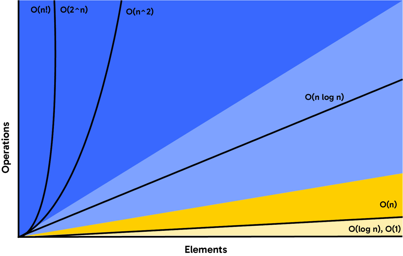
The Big O chart explains that O(1) or constant time is ideal, meaning the algorithm runs a single step. O(log n) is also efficient, among other time complexities shown.

• O(1) - Excellent

• O(log n) - Good

• O(n) - Fair

• O(n log n) - Bad

• O(n^2), O(2^n) and O(n!) - Worst

If the calculation doesn’t change with more input, it's constant time (O(1)). If the input is halved at each step, it's logarithmic (O(log n)). A single loop means linear time (O(n)). Two loops inside each other are quadratic time (O(n^2)). And if each new input doubles the work, that's exponential time (O(2^n)).

Big O Time Complexity with Examples

1. Constant Time O(1)

An algorithm has a constant time complexity as O(1) when there is no dependency on the input size. Here, the execution time is always the same irrespective of the input size.

Example - Checking whether a number is odd or even

number = 15

if number % 2 == 0:

print("Even")

else:

print("Odd")

1. Linear Time Complexity O(n)

An algorithm where the operations increase with the linear increase in the number of inputs is known to have linear time complexity. In short, the time taken is directly proportional to the size of the input.

Example - Linear Search

def linear_search(arr, target):

for i in range(len(arr)):

if arr[i] == target:

return i

return -1

array = [5, 3, 8, 6, 7, 2]

print(linear_search(array, 6)) # Returns the index of 6

1. Logarithmic Time Complexity O(log n)

Cases where the operation of the algorithm is reduced by a fraction(usually half) is considered to have a logarithmic time complexity, also known as divide and conquer strategies.

Example - Binary Search in a Sorted Array

def binary_search(arr, target):

low, high = 0, len(arr) - 1

while low <= high:

mid = (low + high) // 2

if arr[mid] == target:

return mid

elif arr[mid] < target:

low = mid + 1

else:

high = mid - 1

return -1

array = [1, 2, 4, 5, 8, 10]

print(binary_search(array, 5)) # Returns index of 5

1. Quadratic Time O(n^2)

When the time taken by an algorithm is proportional to the square of the input size, it is known to exhibit quadratic time complexity. Usually this is often seen in nested iterations.

Example - Checking for duplicates in an Array

def contains_duplicate(arr):

for i in range(len(arr)):

for j in range(i + 1, len(arr)):

if arr[i] == arr[j]:

return True

return False

array = [1, 2, 3, 4, 5, 1]

print(contains_duplicate(array)) # Returns True

1. Exponential Time Complexity O(2^n)

When an algorithm's runtime doubles with the addition of each input it is known to exhibit exponential time complexity. This is common in algorithms that involve recursive calls with multiple branches. This is because the algorithm explores every permutation or combination of the input data.

Example - Time Complexity Analysis of Fibonacci Series

def fibonacci(n):

if n <= 1:

return n

else:

return fibonacci(n-1) + fibonacci(n-2)

print(fibonacci(10)) # Calculates the 10th Fibonacci number

1. Linearithmic Time Complexity O(n log n)

This type of time complexity combines linear and logarithmic behaviour. It’s most commonly observed in divide and conquer algorithms or efficient sorting algorithms.

Example - Time Complexity Analysis of Quick Sort

def quick_sort(arr):

if len(arr) <= 1:

return arr

else:

pivot = arr[0]

less = [x for x in arr[1:] if x <= pivot]

greater = [x for x in arr[1:] if x > pivot]

return quick_sort(less) + [pivot] + quick_sort(greater)

array = [10, 7, 8, 9, 1, 5]

sorted_array = quick_sort(array)

print("Sorted array:", sorted_array)

1. Factorial Time Complexity O(n!)

Factorial time complexity occurs when the number of operations increases factorially with the size of the input data. It is commonly seen in algorithms that need to generate all possible permutations or combinations of the input data.

Example - Generating all permutations of a string

from itertools import permutations

def all_permutations(s):

return [''.join(p) for p in permutations(s)

print(all_permutations("abc")) # Prints all permutations of "abc”

These are the most common time complexities that one can encounter while working with algorithms.

What are some other examples that you can think of for the various types of Time complexities?

With HeyCoach’s structured DSA and System Design Course learners are able to understand Time Complexity and complex DSA topics with ease. These topics are covered by MAANG coaches who give you insights about different projects that product companies work on. To know more, click here.